01-04-2012, 06:00 PM
Dear Seb,
Please could you upload the VEDA templates that are not working as expected?
Theb I will take a look.
Thanks,
Mauri
Veda2.0 Released!
|
ELC Car as night storage technology
|

01-04-2012, 06:00 PM
Dear Seb,
Please could you upload the VEDA templates that are not working as expected? Theb I will take a look. Thanks, Mauri
02-04-2012, 02:10 PM
Hi Antti, hi Maurizio, thanks a lot for your help. I did not manage the copy the processes into other models. Even when I took Antti’s test model and changed the TimeSlices, not all Processes would work. (See attached example, it contains the same model with changed TimeSlices). At the moment I solved my problem the following way: I adjusted the TEST model and choose two of the StorageProcesses then copied my entire model (250 processes) into it. This works, but is only a work around. I will go back to this problem later, because I want to understand the reasons. Thanks for your help, I think for the moment I solved (worked around) my problem. Seb uploads/71/STEMMarch12.zip
24-11-2014, 07:47 AM
Dear Antti Apologies to pick up on an old thread, but I have been trying to model plug-in hybrid vehicles in an identical manner to the test model you gave above. However when I uploaded and ran the model from your post above, the results didn't seem right. Only one of the 5 technologies you include use both ELC and GSL - most rely upon ELC only, which doesn't represent plug-in hybrids particularly well. Ideally I would like to use the DAYNITE - DAYNITE option (so the NSTCAR-DD technology) as this suits our needs best. I include a screenshot below to show the results. Has something changed in the TIMES code that means the attached no longer functions as needed? Thanks for any help Christophe 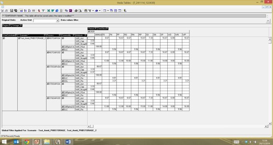
24-11-2014, 01:16 PM
The image you provided is so blurred, that I cannot really see the details, sorry. However, quoting myself from an earlier post in this thread: "Finally, I included also an additional variant of the ANNUAL-ANNUAL level NST process, which has also a FLO_SHARE parameter constraining the share of electricity in the total fuel input. These kind of share constraints can only be specified for normal processes, and therefore I think the ANNUAL-ANNUAL alternative may actually be considered the best one for practical modeling of plug-in hybrid cars. For this variant, you can even specify constraints on the fraction of charging that can occur at different timeslices (as demonstrated in my earlier DemoPlugin example)." I guess you are seeing the GSL used by this normal process mentioned above? As you can see, I was specifically noting that one cannot directly model such input share constraints for genuine storage processes. You can model them for dummy auxiliary storage flows if you introduce such, but that would become a bit ugly, and was therefore left to the reader as an exercise. The whole point of my example was to demonstrate that using the ANNUAL level NST process approach is, in my opinion, useful. I don't know why you would like to use the DAYNITE-DAYNITE option. Maybe you can explain that? But if that's what you want, you would apparently need auxiliary flows for the share constraints.
24-11-2014, 02:44 PM
Dear Antti Many thanks for your response. Apologies that the screenshot is
so small - hopefully the one below is better. It is clear from what you now say that there is no GSL input to any process
other than STDCAR+DA because only this technology has a fixed share constraint.
Since all of the other technologies do not use any GSL, they are acting much
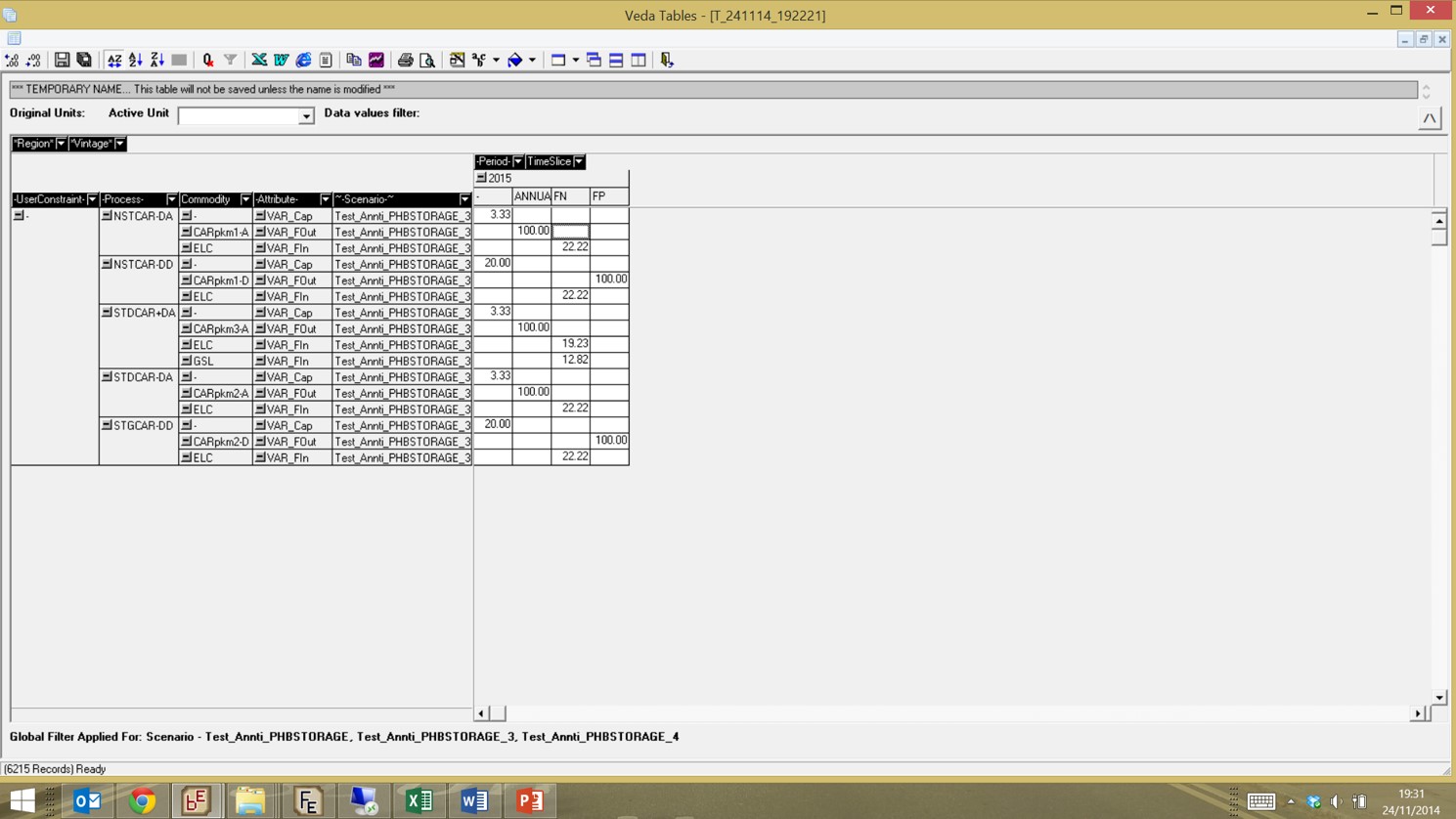
more as pure battery electric vehicles rather than PHEV, and so none are really suitable for modelling PHEV and are best avoided. The reason for using DAYNITE-DAYNITE was mainly because, although you note above that: “Using DAYNITE level demand and a DAYNITE level car technology is not necessary for the modeling of demand load curves and the use of cheap off-peak electricity. That can be done equally well with an ANNUAL level NST technology.” It is not clear to me that this is the case. The model does not appear to be take account of the COM_FRs specified for the demand quantity unless it is specified at the DAYNITE level. For example, the model does construct sufficient capacity to satisfy the demands in individual timeslices unless they are specified as DAYNITE. I have run the model again to try to demonstrate this as shown below. In
this version everything is identical except all of the demand occurs in the FP
timeslice and is zero elsewhere (i.e. COMFR~FP = 1). We can see that there is a
large difference in the capacities constructed between those that specify the
demand on an annual basis (NSTCAR-DA, STDCAR+DA, and STDCAR-DA) and those that do it on a
DAYNITE basis (NSTCAR-DD, STGCAR-DD). If the model was taking into account the
COM_FR, I would expect the capacity to be 20 as it is for the DAYNITE specification. There also appears to be another problem when specifying the output commodity at an
annual level and the technology at a DAYNITE level. The model appears to be able to input
the feedstock in a given time slice and
output the product in a different time slice, so long as these properly balance
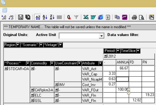
on an annual level. This can be seen in the example below in STDCAR+DA, GSL goes in FN but the demand is obviously all in FP as before. While this doesn't matter in particular for this example (as
petrol can be stored), for electricity in non-storage technologies this is
important. Technologies specified in a similar way can switch away from consuming
electricity in any given time slice so long as they increase consumption in a
different time slice. This is often not desirable. Specifying demands at the DAYNITE
level removes this flexibility as the model is forced to consume the
electricity in the timeslice it produces the output. Finally, although not as importantly, since we have specified
COM_FRs for the output commodity, it is sometimes useful to see this shaping of
demand in the results which is not possible by using an annual commodity. For these reasons, since we are specifying the commodity at the
DAYNITE level, I thought it necessary also to specify the technology as
DAYNITE. Is there something I have missed something here? Thanks Christophe
I think you are missing quite a lot here. Please find my quick answers below (referring to your statements by SN and to my answers by AN):
S1: Since all of the other technologies do not use any GSL, they are acting much more as pure battery electric vehicles rather than PHEV, and so none are really suitable for modeling PHEV and are best avoided. A1: Not true. I think I clearly explained how you can define any necessary share constraints even for the inputs of genuine storage processes. So, there is no reason to avoid these modeling approaches as such, if you really need to optimize the activities of car technologies among timeslices. I would only be curious to know, whether you would really need that? S2: The model does not appear to be take account of the COM_FRs specified for the demand quantity unless it is specified at the DAYNITE level. For example, the model does construct sufficient capacity to satisfy the demands in individual timeslices unless they are specified as DAYNITE. A2: I can only disagree. If I specify an annual availability of 20,000 km/a for the car technology, meaning that the annual "mileage" is 20,000 vkm (vehicle-km), the capacity of the technology will accurately reflect this annual availability, regardless of the distribution of the vkm across the timeslices. This is exactly what I would expect. Do you expect the annual mileage to be different with different COM_FR, even if you have specified it with NCAP_AFA? S3: If the model was taking into account the COM_FR, I would expect the capacity to be 20 as it is for the DAYNITE specification. A3: I disagree. COM_FR and NCAP_AFA are both exogenous input parameters. If you specify the ANNUAL mileage to be 20,000 vkm/car (as in my example), one would certainly expect that much of ANNUAL vkm/car in the results. The demand being 100 Mpkm and the amount of pkm/vkm is 1.5, and CAPACT=0.001, the expected capacity needed is 100/1.5/20000/0.001 = 3.3333, just as shown in the results. If you want to define a different annual mileage for the car, you can simply change the annual availability. S4: There also appears to be another problem when specifying the output commodity at an annual level and the technology at a DAYNITE level. The model appears to be able to input the feedstock in a given time slice and output the product in a different time slice, so long as these properly balance on an annual level. A4: This is not a problem. The technology is by definition a night storage technology, and therefore you can obviously load the car with fuel in the night, and drive during the day. And there is NO such storage capability on the WEEKLY or SEASON level. Thus, GSL and ELC can of course be loaded in FN while the demand is in FP (it is the same day). Moreover, as I have also mentioned, the DAYNITE charging fractions can also be constrained according to timeslice. S5: While this doesn't matter in particular for this example (as petrol can be stored), for electricity in non-storage technologies this is important. Technologies specified in a similar way can switch away from consuming electricity in any given time slice so long as they increase consumption in a different time slice. S6: Finally, although not as importantly, since we have specified COM_FRs for the output commodity, it is sometimes useful to see this shaping of demand in the results which is not possible by using an annual commodity. I hope you can respond to my answers and clarify your point of view further. And, if you have suggestions for improving TIMES, they are also always welcomed, especially if you can formulate them in math terms.
25-11-2014, 07:39 AM
(This post was last modified: 25-11-2014, 07:42 AM by cmcglade_UCL.)
A1: Not true. I think I clearly explained how you can define any necessary share constraints even for the inputs of genuine storage processes. So, there is no reason to avoid these modeling approaches as such, if you really need to optimize the activities of car technologies among timeslices. I would only be curious to know, whether you would really need that? I had, perhaps naïvely, assumed that by your generating some technologies, which you refer to as PHEV, that they properly represented how PHEV actually operate. Nowhere in your post on 30th March 2012 did you mention that these were only “half completed” and that the user would need to put in additional share constraints to make them operate as would normally be expected for PHEV. In my post I therefore thought it would be useful to any future readers to mention this so that they do not expect, as I did, that these technologies would properly represent the way a PHEV operates. A2: I can only disagree. If I
specify an annual availability of 20,000 km/a for the car technology, meaning
that the annual "mileage" is 20,000 vkm (vehicle-km), the capacity of
the technology will accurately reflect this annual availability, regardless of
the distribution of the vkm across the timeslices. This is exactly what I would
expect. Do you expect the annual mileage to be different with different COM_FR,
even if you have specified it with NCAP_AFA? A3: I disagree. COM_FR and NCAP_AFA are both exogenous input parameters. If you specify the ANNUAL mileage to be 20,000 vkm/car (as in my example), one would certainly expect that much of ANNUAL vkm/car in the results. The demand being 100 Mpkm and the amount of pkm/vkm is 1.5, and CAPACT=0.001, the expected capacity needed is 100/1.5/20000/0.001 = 3.3333, just as shown in the results. If you want to define a different annual mileage for the car, you can simply change the annual availability. If all of the demand is in a single timeslice, then expected capacity is 100/1.5/20000/0.001 * 12 (the length of time in the timeslice) / 2 (the time slice-specific activity factor) = 20. This is what we see in my previous screenshot for the technologies that have the demand commodity at a DAYNITE level. As that shows, your model gives different capacities depending on whether the demand is specified at ANNUAL level or the DAYNITE level. When COM_FRs are specified, we obviously want the model to take these into account, and if the model WAS appropriately taking them into account when demand is at an ANNUAL level then I would have expected all of the technologies to have a capacity of 20. The model is not doing this. Therefore the COM_FRs are not doing anything if the demand is at an ANNUAL level. Are you therefore saying that if we want to specify demands at the ANNUAL level but also have demand load varying over a day then we MUST specify some other parameters at the timeslice level (probably the availability factor) and the COM_FRs are redundant? As a side point, in your previous post, you mentioned that these four technologies were “basically all equivalent”. It is now evident that you must have meant that they are equivalent for the very specific parameters, including the COM_FRs, that you specified. By changing some of the COM_FRs the four technologies are now NOT “basically all equivalent”, as shown in the previous example. One must therefore be very careful to ensure that the correct specification is used and, to be able to examine that the model is behaving as expected, I suspect it is thus easiest to specify the commodity at a DAYNITE level. A4: This is not a problem. The
technology is by definition a night
storage technology, and therefore you can obviously load the car with
fuel in the night, and drive during the day. And there is NO such storage
capability on the WEEKLY or SEASON level. Thus, GSL and ELC can of course be
loaded in FN while the demand is in FP (it is the same day). Moreover, as I
have also mentioned, the DAYNITE charging fractions can also be constrained
according to timeslice. The example I gave was unfortunate as I can see how you might think that GSL input during FN results from the fact that the technology is a night storage technology. I attach another screenshot from a different year which shows GSL going in in FD not in FN. If STDCAR+DA was acting only as a night storage technology, then GSL should not be able to go in during FD and the output produced in FP. I would be grateful if you could explain why this is possible.
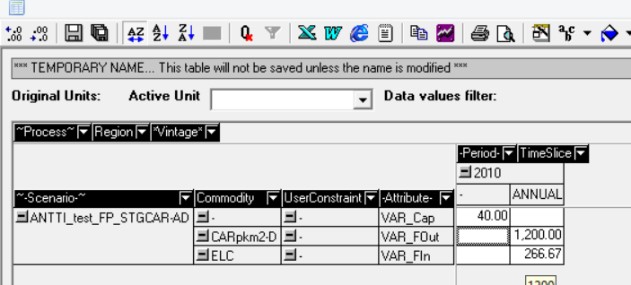
A6: You could define the output commodity on the DAYNITE level for that, if you like, while keeping the technology at ANNUAL. So, I don't see any issue here either. Is this as trivial as you make it sound? I am not sure it is, as I think this would also change results. To demonstrate this, take my example where all of the demand is in FP, but also change the technology STGCAR-DD from operating on the DAYNITE level to the ANNUAL level. I called this scenario ANTTI_test_FP_STGCAR-DA with the outputs are shown below. In this, the technology is producing an output of 1200 as it must spread it out evenly across all timeslices (which are in periods of 1/12 so 1200/12 satisfies the demand of 100 in FP). I suppose it may be possible to change how this technology operates, but I don’t know how to do this. Further, given that reproducibility is important for getting others to understand how a model is functioning, I would rather avoid having to specify different technologies in numerous different ways for no real benefit. Many thanks for your help
Thanks for elaborating your concerns further. Here are my responses: A1: Had you been reading the original posts and example model by Seb, to which my examples were a response, you would have seen that there were no share constraints in Seb's original example. Seb had some problems with getting the NST processes work, and I tried to help by providing a set of working examples. Seb was not asking about the share constraints; only you are now. But I am wondering, how you could possibly think that the processes would be using both ELC and GSL realistically without defining any share constraints? A2: You seem to be still missing the point. When not optimizing the process activities, the resulting annual mileage is an exogenous assumption. It is an exogenous assumption in the DAYNITE process, just like you demonstrated by your formula 100/1.5/20000/0.001 * 12 / 2. For the DAYNITE process, it all boils down to the timeslice-specific factor 2, which results in an annual mileage of 3,333 vkm with you new test load curve. If you change the availability factor, you will get a different annual mileage. Now, if 3,333 vkm is really the annual mileage that you consider correct for the process, you should just define that as the AFA accordingly: AFA=3333.33. And then you have no problem! It is as simple as that, and so I cannot see how this could be a problem with the ANNUAL level technology: If the activities are not optimized, you will always know what the annual utilization factor (AFA) should be, and you can thus define the max. utilization factor accordingly. Can you explain where the problem is with that? A4: Ok, so you have a very strict definition of night storage: You assume that the charging should be possible only at some timelices that have been defined as "night". I would think that there is no technical reason why the charging could not occur at any hour of the day, and that's how the ANNUAL level NST works: it can optimize the charging at cheap off-peak hours (and these are just being called "night") regardless of the time of the day they actually occur. I cannot see any reason why the battery should be forced to be charged in the true night-time, if the prices happen to be high during the night. Thus, GSL going in at FD (daytime) is of course equally possible as at FN with respect to the technical characteristics of the daily storage. But again, it is extremely easy to bind the daytime charging flows to zero, if you think that charging is technically impossible at cheap daytime hours! So, again I don't see where the problem is; can you explain? A6: It seems you are not familiar with the corresponding TIMES reporting option. Try setting the "TS for flow reporting" to "Commodity level" in the VEDA Control Panel. I find it very useful myself. [EDIT]: You also say: "Therefore the COM_FRs are not doing anything if the demand is at an ANNUAL level." This is nonsense. I am usually having all my demands at the ANNUAL level in my models, and the resulting load curves are perfect. For the ANNUAL NST storage, COM_FR defines the WEEKLY/SEASON load curve, and is thus necessary for the correct modeling of the technology. If you would define all demands and demand technologies at the DAYNITE level, you would basically need a vast amount of additional daynite AF parameters to ensure that each technology operates realistically. That's why I prefer to use ANNUAL level demands and ANNUAL level demand technologies. They do work very well.
25-11-2014, 03:12 PM
A2: You seem to be still
missing the point. When not optimizing the process activities, the
resulting annual mileage is an exogenous
assumption. It is an exogenous assumption in the DAYNITE process, just
like you demonstrated by your formula 100/1.5/20000/0.001 * 12 / 2. For the
DAYNITE process, it all boils down to the timeslice-specific factor 2, which
results in an annual mileage of 3,333 vkm with you new test load curve.
If you change the availability factor, you will get a different annual mileage.
Now, if 3,333 vkm is really the annual mileage that you consider correct
for the process, you should just define that as the AFA accordingly:
AFA=3333.33. And then you have no problem! It is as simple as that, and
so I cannot see how this could be a problem with the ANNUAL level technology:
If the activities are not optimized, you will always know what the annual
utilization factor (AFA) should be, and you can thus define the max.
utilization factor accordingly. Can you
explain where the problem is with that? Of course the annual mileage is an exogenous assumption, however this is
usually based on real world data. It would therefore be preferable to at least
use this exogenous assumption figure consistently. Your edit implies that to take
account of the COM_FRs when the commodity is ANNUAL you must modify the
exogenously-assumed annual activity factor (in this case 20,000) by the
duration of the modelling timeslice and the COM_FRs. It would be difficult to
anyone trying to understand what the model attributes actually mean if it
requires all of this modification. To do this, it appears to me that you must multiply this AFA by max(timeslice
duration * AF / COM_FR) calculated for each timeslice where COM_FR > 0. So
in the above example the AFA would be changed to 20000* (1/12*2/1) = 3,333. If,
on the other hand COM_FR was 0.5 in a given timeslice and 0.25 in two others,
the AFA would need to be multiplied by (1/12*2/0.5) to give 6,666. One must
then do this for all technologies that can satisfy the demand. Alternatively
you could modify the AF for each specific timeslice, but this would be the same
amount of work. You state that in your model “all my
demands at the ANNUAL level in my models, and the resulting load curves
are perfect”. As you stated in your last post, if you specify the
commodity at an ANNUAL level you cannot see if the load curve is “perfect”. Therefore
the easiest way to see if the COM_FRs are working is if the model installs sufficient
capacity to satisfy the demand in a given timeslice. In the examples that I
have previously attached, the model has not installed sufficient capacity to satisfy
the COM_FRs, so they are clearly not acting “perfectly”. If you could attach an
example that clearly shows that an ANNUAL commodity takes into account specified
COM_FRs that would be appreciated. As I just mentioned, I suspect this will
require reformulating AFA or AF off model to match what the COM_FRs represent.
If that is the case, then this is fine, but it would be helpful to say this explicitly.
A6: It seems you are not familiar
with the corresponding TIMES reporting option. Try setting the "TS for
flow reporting" to "Commodity level" in the VEDA Control Panel.
I find it very useful myself. 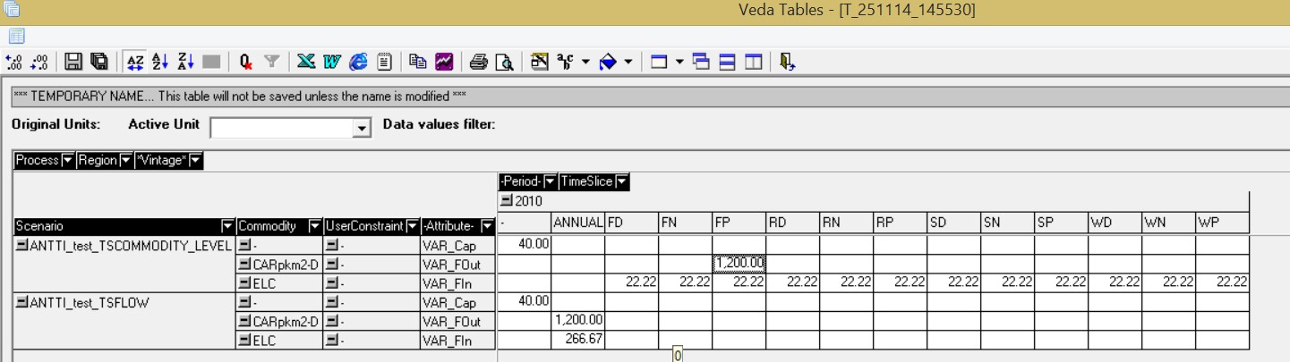 Many thanks for your additional clarifications. Please find my responses below: A2: In my view, the annual mileage (e.g. 20,000 vkm) is far more transparent than the arbitrarily chosen value of 2.0 for the timeslice-specific availability factor. Hence, I find it transparent and useful to define, in the first place, the annual mileages for the car technologies. We have good statistics for the average value of that parameter, and so the values have a good statistical basis. On the other hand, we don't have good statistics for timeslice-specific car availabilities, on which you seem to put all the importance, because your annual mileage under the new load curve case is completely based on that arbitrary value! Therefore, I find it much more transparent to use the annual mileage as the primary input data. When it is specified for the technologies, the ratio between the annual activity and the capacity will thus be always correctly modeled in accordance with real-world driving patterns, and it is also very transparent. Of course, I also define the load curve by using COM_FR, which is less firmly based on real data, as the statistics on hourly transport volumes are not that good. However, of course these two parameters must be consistent with each other. You seem to claim that doing what I describe above would lead to some modeling problems. I cannot myself see any notable problem in it, and neither have your various explanations convinced me that this would be the case. You are basing your arguments on suddenly changing the load curve to a very hypothetical one, which would not conform to any typical use of a car. But if it would, you would of course also have an annual mileage estimate for such usage pattern, no? And then you should of course update the annual mileage parameter at the same time. Concerning the load curves, the only reliable way to verify them working is to look at the distribution of the input flows. For non-storage demand technologies, that distribution follows exactly the load curve, which demonstrates that the load curves are fully working when using ANNUAL level demand technologies. For daily storage technologies, the daily distribution of the inputs of course does not follow the load curve, but the WEEKLY and SEASON curves are fully reproduced. On the other hand, if you model all the technologies at the DAYNITE level, it will be much more difficult to reproduce the load curves in the input flows, as they normally should. A6: Your example, which you kindly named after me, is simply not sensible. Modeling a genuine timeslice storage at the ANNUAL level makes no sense at all, irrespective of the level of the demand commodity, and so you why are you deliberately using such a crafted example? Why don't you present a case for some sensibly defined process instead? It would be much more useful for the discussion, if you find a technology working unexpectedly.
26-11-2014, 05:38 AM
Some further corrections to your many incorrect statements: 1) You say: "As you stated in your last post, if you specify the commodity at an ANNUAL level you cannot see if the load curve is “perfect”." I have not stated anything like this. Where do you get such an incorrect idea? You can certainly verify the that the load curve is perfect by looking at the distribution of the input flows. 2) You say: "Your edit implies that to take account of the COM_FRs when the commodity is ANNUAL you must modify the exogenously-assumed annual activity factor (in this case 20,000) by the duration of the modelling timeslice and the COM_FRs. It would be difficult to anyone trying to understand what the model attributes actually mean if it requires all of this modification." This is again very incorrect. I have only said that if you really think that the annual mileage of a car should be 3,333 vkm, then you should update the AFA parameter to reflect this. But it is only you who are claiming that the annual mileage should be 3,333 vkm with your test load curve, because you have claimed that the correct capacity should be 20. Your new annual mileage would obviously be inconsistent with real-world data, assuming that the original annual mileage was indeed consistent. So, in your modeling approach, you basically assume that whenever you update your load curves e.g. with improved estimates for the time distribution of the transport volumes, your annual mileage should change in the model results! In my view this is totally nonsensical, because you have good estimates on the annual mileage, based on real-world data. But you claim that the correct mileage should change in the model from those real-world estimates, just because you have updated your load profile with some new estimates. That kind of modeling makes little sense to me, because it would no longer produce correct capacities that would reflect the real-world data. You essentially seem to think that the load curves determine the required capacity. That is not the case: the load curves only define the load profile, they do not give the utilization factors of the technologies producing the demand commodity.
26-11-2014, 09:05 AM
Anitti, It’s clear that we continue to talk at cross purposes. This conversation is therefore unlikely to help resolve the problems we are having or be of any help to future readers. As a side point, responding antagonistically, which is unfortunately common on this forum, is not particularly helpful to developing an effective setting in which other users feel comfortable with raising issues and problems they are facing. |
|
« Next Oldest | Next Newest »
|